Automated Calibration Injection

In this section, the automated calibratoin injection in xpdAcq will be introduced.

CalibPreprocessor

The CalibPreprocessor takes care of the injection of calibration data into the data stream.

It is registered in the xrun.calib_preprocessors list.

xrun.calib_preprocessors

[<CalibPreprocessor of detector with 0 cache>,
 <CalibPreprocessor of detector1 with 0 cache>,
 <CalibPreprocessor of detector2 with 0 cache>]

Logic

When CalibPreprocessor finds that the detector is going to be triggered and it is not a dark frame (not labeled by dark_group_prefix), it will start doing its job. What it will do is presented as the peseudo below.

if (there are no registered `locked_signals`):
    inject the calibration data collected when there were no `locked_signals`
else:
    read the `locked_signals` and search the cache
    if (there is calibration data collected at the same values of the `locked_signals`):
        inject that calibration data
    else:
        inject the most recent calibration data

Here, the locked_signals can be any scalar values that determines the geometry of the setup, like the z axis motor of the detecotr, the z axis motor of the sample stage, etc.

For example, the locked_signals is [det_stage_z], which is the motor of the z axis of the detector. And the CalibPreprocessor has det_stage_z=200 -> calibration data 1 and det_stage_z=1000 -> calibration data 2 in the cache. The latter record is the latest record. When the detector is at position det_stage_z=200, the CalibPreprocessor will inject the calibration data 1 into the data stream and then the the detector moves to position det_stage_z=1000, the CalibPreprocessor will inject calibration data 2 into the data stream. After that, the detector moves to det_stage_z=1200. There is no record at 1200 and the CalibPreprocessor will inject the latest calibration data 2 into the data stream. This behavior is designed to be coherent with the old xpdAcq calibration logic, that is, always injecting the lastest calibration data without checking the situations.

Run Calibration

CalibPreprocessor is only in charge of injecting calibration data. To run the calibration and give the calirbation result to CalibPreprocessor, RunCalibration functor should be used.

This functor is usually set up during the start up of the ipython session and its variable name is usually run_calibration.

run_calibration()

What it does is as following:

1. Let the xrun collect a image and send it to the analysis server.

2. The analysis server will start the calibration session and the user will interact with the pyFAI-calib2.

3. Wait for the calibration to be finished.

4. Once it is finished, load the calibration data from the output poni file.

5. Let xrun read the locked_signals and add the mapping from locked_signals values to the calibration data into the cache.

To know more about how to interact with pyFAI-calib2, here is a cookbook for it.

There could be multiple detectors. Each detector has a Calibpreprocessor to look after it. The run_calibration will calibrate the detecotr taken care by the first CalibPreprocessor by default.

xrun.calib_preprocessors[0]

<CalibPreprocessor of detector with 0 cache>

To calibrate another detector, use the key word arguemnt preprocessor_id. It is the index of the CalibPreprocessor in the xrun.calib_preprocessors. For example, to calibrate the detector taken care by the second CalibPreprocessor, which has the index 1 in the list, use preprocessor_id = 1.

run_calibration(preprocessor_id=1)

Locked_signals

In default, the motors control the z axis positions of detecotrs have already been registered in the CalibPreprocessor in the ipython start up session. For example, the first CalibPreprocessor has the det_stage_z as the locked signal.

xrun.calib_preprocessors[0].locked_signals

[SoftPositioner(name='det_stage_z', parent='det_stage', settle_time=0.0, timeout=None, egu='mm', limits=(0, 0), source='computed')]

Users can remove it or add new locked_signals by usual python list operation. For example, to pop the det_stage_z.

det_stage_z = xrun.calib_preprocessors[0].locked_signals.pop()

And add this motor back to the list.

xrun.calib_preprocessors[0].locked_signals.append(det_stage_z)

Calibration Data from Poni Files

CalibPreprocessor can also read the calibration data from the poni files and add it into the cache. There are two ways to do it. First way is to use load_calib_result. It is used when users would like to manually specify what locked_signals it should be when this calibration data is injected.

Below is an example to use the calibration data in the “near_field.poni” when the det_stage_z is at 200 mm.

cpp0 = xrun.calib_preprocessors[0]

cpp0.load_calib_result({"det_stage_z": 200.}, "near_field.poni")

The data will be record in the cache.

cpp0._cache

OrderedDict([(frozendict.frozendict({'det_stage_z': 200.0}),
              (1.671e-11, 0.2, 0.2, 0.2, 0.0, 0.0, 0.0, 'Perkin detector'))])

Here, we clear the cache because we will demonstrate a second example.

cpp0.clear()

The second way is to use the calibration data in the poni at the current locked_signals values. Below is an example to use the calibration data at the current det_stage_z position. Currently the position is 0.0.

calib_data = cpp0.read("near_field.poni")
xrun({}, cpp0.record(calib_data))

()

In this way, the calibration data will be record with the key of the current det_stage_z position 0.0.

cpp0._cache

OrderedDict([(frozendict.frozendict({'det_stage_z': 0.0}),
              (1.671e-11, 0.2, 0.2, 0.2, 0.0, 0.0, 0.0, 'Perkin detector'))])

This is equivalent to manually read the det_stage_z and add the calibration data. Its advantage is to make sure every operation command on the devices go throught the xrun.

cpp0.load_calib_result({"det_stage_z": det_stage_z.get()}, "near_field.poni")

Here, we clear the cahce to preprare for the next example.

cpp0.clear()

Enable and Disable

The CalibPreprocessor can be disabled by calling disable.

xrun.calib_preprocessors[0].disable()

It can be enabled again by calling enable.

xrun.calib_preprocessors[0].enable()

Calibration Data Stream

The calibration data is saved in the calib data stream. For example, we collect a image on the detector.

xrun(0, 1)

INFO: requested exposure time = 0.1 - > computed exposure time= 0.1
INFO: Current filter status
INFO: flt1 : In
INFO: flt2 : In
INFO: flt3 : In
INFO: flt4 : In


Transient Scan ID: 2     Time: 2022-04-13 16:43:32
Persistent Unique Scan ID: 'eb975d15-2531-49ee-8cde-d39c7518cffa'
WARNING: Cannot find 'frozendict.frozendict({'det_stage_z': 0.0})' in the cache. Use the latest one.
New stream: 'calib'
New stream: 'dark'
New stream: 'primary'
+-----------+------------+
|   seq_num |       time |
+-----------+------------+
|         1 | 16:43:32.4 |
+-----------+------------+
generator count ['eb975d15'] (scan num: 2)

('eb975d15-2531-49ee-8cde-d39c7518cffa',)

The calibration data is the calib stream in the database record.

run = db[-1]
run.stream_names

['calib', 'primary', 'dark']

Disposable Calibration Data

All the calibration data in the registered CalibPreprocessors are intended to be used during the whole beamtime. If users would like to use some calibration data just for one specific experiment and dispose it after that, they can provide the keyword argument poni_file.

xrun(
    0, bp.count([detector]),
    poni_file=[(detector, "specific_calibration.poni")]
)

Here, users need to specify the path of the calibration data file, that is, "specific_calibration.poni", and what detector they would like to use this file for, that is, detector. They can specify calibration data for more than one detector when using multiple detectors.

xrun(
    0, bp.count([detector1, det_stage2]),
    poni_file=[
        (detector1, "specific_calibration_1.poni"),
        (detector2, "specific_calibration_1.poni"),
    ]
)

Collecting XRD and PDF by Moving the Detector

Here, an example of collecting XRD and PDF by moving one detector in z axis is shown to demonstrate how the CalibPreprocessor works. Below is the user’s plan. The user wants to collect a near field image for PDF data and a far field image for XRD data for sample 0 at 300 K, 400 K and 500 K. The near field image is taken at det_stage_z = 200 mm while the far field image is taken at det_stage_z = 1000 mm.

plan = bp.list_grid_scan([detector], cryostream, [300., 400., 500.], det_stage.z, [200., 1000.])

The user move the det_stage_z to do the calibration at two different detector positions.

xrun({}, bp.mv(det_stage_z, 200.))
run_calibration()

xrun({}, bp.mv(det_stage_z, 1000.))
run_calibration()

If the user already has the poni files, the user can also directly use them like below.

cpp0 = xrun.calib_preprocessors[0]

cpp0.load_calib_result({"det_stage_z": 200.}, "near_field.poni")

cpp0.load_calib_result({"det_stage_z": 1000.}, "far_field.poni")

Now, there are two calibration data records in the cache.

cpp0._cache

OrderedDict([(frozendict.frozendict({'det_stage_z': 200.0}),
              (1.671e-11, 0.2, 0.2, 0.2, 0.0, 0.0, 0.0, 'Perkin detector')),
             (frozendict.frozendict({'det_stage_z': 1000.0}),
              (1.671e-11, 1.0, 0.2, 0.2, 0.0, 0.0, 0.0, 'Perkin detector'))])

Then, the user starts the plan. The calibration data will be automatically injected to to data stream when the plan is running. What data will be injected is determined by the value of the locked_signals.

xrun.calib_preprocessors[0].locked_signals

[Signal(name='det_stage_z', parent='det_stage', value=0.0, timestamp=1649882537.696865)]

The user execute the plan.

xrun(0, plan)

INFO: Current filter status
INFO: flt1 : In
INFO: flt2 : In
INFO: flt3 : In
INFO: flt4 : In


Transient Scan ID: 3     Time: 2022-04-13 16:44:57
Persistent Unique Scan ID: 'be8310db-452c-4002-8e1b-1a7df291b635'
New stream: 'calib'
New stream: 'dark'
New stream: 'primary'
+-----------+------------+-------------+-------------+
|   seq_num |       time | temperature | det_stage_z |
+-----------+------------+-------------+-------------+
|         1 | 16:44:57.5 |     300.000 |     200.000 |
|         2 | 16:44:57.7 |     300.000 |    1000.000 |
|         3 | 16:44:57.9 |     400.000 |     200.000 |
|         4 | 16:44:58.0 |     400.000 |    1000.000 |
|         5 | 16:44:58.2 |     500.000 |     200.000 |
|         6 | 16:44:58.3 |     500.000 |    1000.000 |
+-----------+------------+-------------+-------------+
generator list_grid_scan ['be8310db'] (scan num: 3)

('be8310db-452c-4002-8e1b-1a7df291b635',)

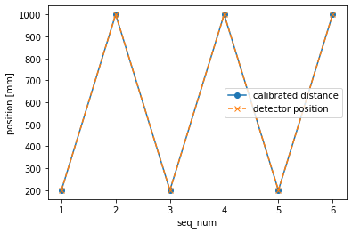
There is New stream: 'calib' craeted. This stream is where the calibration data is saved. Below is a visualization of the calibrated distances and the detector position on z axis. The recorded calibrated distance changes with the position of the detector.

import numpy as np
import matplotlib.pyplot as plt


def visualize(run):
    dist = np.array(list(run.data("detector_dist", stream_name="calib"))) * 1000
    det_z = np.array(list(run.data("det_stage_z", stream_name="primary")))
    seq_num = list(range(1, len(dist) + 1))
    _, ax = plt.subplots(figsize=(6, 4))
    ax.plot(seq_num, dist, "-o", label="calibrated distance")
    ax.plot(seq_num, det_z, "--x", label="detector position")
    ax.set_xlabel("seq_num")
    ax.set_ylabel("position [mm]")
    ax.legend()
    return

run = db[-1]
visualize(run)